# Analysis Pack
library(tidyverse)
library(tidytuesdayR)
library(scales)
library(infer)
# Theming Pack
library(nationalparkcolors)
library(paletteer)
# Styling Pack
library(reactable)
library(reactablefmtr)
library(showtext)
library(showtextdb)
library(extrafont)
library(extrafontdb)
font_add_google("BenchNine", family = "BenchNine")
showtext_auto()Libraries
Loading in my go-to libraries.
Data
artwork <- readr::read_csv('https://raw.githubusercontent.com/rfordatascience/tidytuesday/master/data/2021/2021-01-12/artwork.csv')
artists <- readr::read_csv("https://github.com/tategallery/collection/raw/master/artist_data.csv")
artwork_artist_tbl <- artwork %>%
left_join(artists, by = c("artist" = "name"), suffix = c("", "_ar_df")) %>%
separate(placeOfBirth, into = c("city", "country"), sep = ", ", extra = "merge")
artwork_artist_tbl %>%
filter(!is.na(country)) %>%
count(country, sort = T) %>%
reactable::reactable(
theme = espn(font_size = 12, centered = TRUE),
columns = list(
country = colDef(name = "Country", align = "center"),
n = colDef(name = "No. of Occurrences", align = "center")
)
)Tate Art Museum is a museum based in the United Kingdom, so I am not really surprised to see the UK arts being reported more frequently in this dataset.
artwork_artist_tbl %>%
  count(country, artist, sort = T) |>
  reactable(
    theme = espn(font_size = 12),

    columns = list(
      country = colDef(name = "Country", align = "center"),

      artist = colDef(name = "Artist", align = "center"),

      n      = colDef(name = "No. of Occurrences", align = "center")
    )
)A lot of the United Kingdom’s records in this dataset comes from Turner, Joseph Mallord William. According to Wikipedia, he was known as romantic painter, print maker, and water colorist. I am googling his paintings right now, and they are something.
Statistical Inference
I am interested in learning more about the average dimension of the arts (average height, width, and depth). I think one way to go about this would be to collect all the arts available in the world and measure their dimension which is not just super expensive but also impossible. Another way to learn about the average dimension of the art would be to create bootstrap resamples and calculate their means.
Assumptions:
- I am assuming this dataset to be randomly sampled, so that any inference made using this sample can be generalized.
- I am assuming this dataset to be representative of all of the art works around the world.
My population parameter of interest is the average dimension of an art which is unknown. However, I have this dataset as a sample. I am going to consider using this sample to create bootstrapped resamples and calculate the average dimension on those bootstrapped resamples. In order to proceed ahead, I am going to use infer for virtual bootstrap simulation and inference. Go check out infer package!!!
Distribution of dimensions from the sample
artwork_artist_tbl %>%
  filter(!is.na(height)) %>%
  ggplot(aes(height)) +
  geom_histogram(color = "white", fill = "#F6955E", alpha = 0.8) +
  scale_x_log10() +
  geom_vline(xintercept = artwork_artist_tbl %>% summarize(avg_height = mean(height, na.rm = T)) %>% pull(avg_height), lty = 2, size = 1.5)+
  theme_minimal()+
  theme(text = element_text(family = "BenchNine"),
        plot.title = element_text(size = 15, face = "bold", hjust = 0.5),
        plot.subtitle = element_text(hjust = 0.5))+
  labs(x = "Height (mm)",
       y = "# of arts",
       title = "Distribution of Height",
       subtitle = "The dashed line represents the average height of art works from original sample i.e. 346.88 mm, and x-axis is log scaled")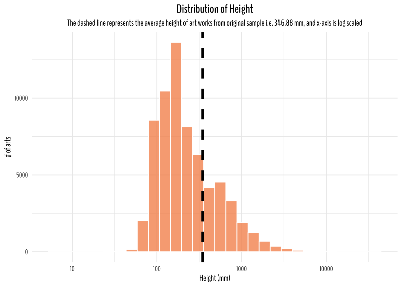
artwork_artist_tbl %>%
  filter(!is.na(width)) %>%
  ggplot(aes(width)) +
  geom_histogram(color = "white", fill = "#F6955E", alpha = 0.8) +
  scale_x_log10() +
  geom_vline(xintercept = artwork_artist_tbl %>% summarize(avg_width = mean(width, na.rm = T)) %>% pull(avg_width), lty = 2, size = 1.5)+
  theme_minimal()+
  theme(text = element_text(family = "BenchNine"),
        plot.title = element_text(size = 15, face = "bold", hjust = 0.5),
        plot.subtitle = element_text(hjust = 0.5))+
  labs(x = "Width (mm)",
       y = "# of arts",
       title = "Distribution of Width",
       subtitle = "The dashed line represents the average depth of artworks from original sample i.e. 323.81 mm, and x-axis is log scaled")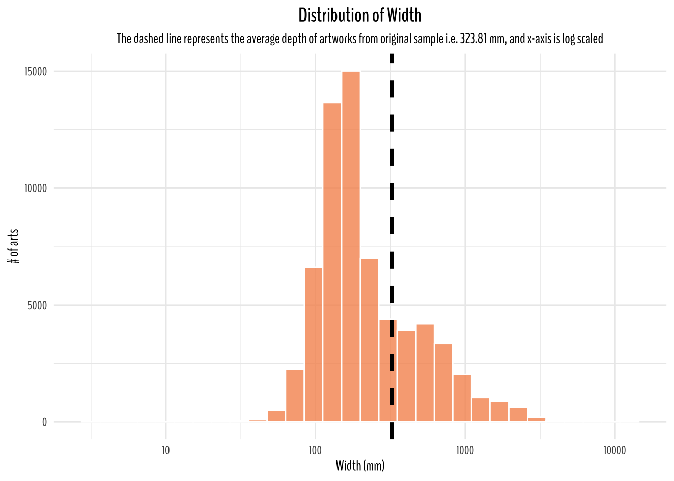
artwork_artist_tbl %>%
  filter(!is.na(depth)) %>%
  ggplot(aes(depth)) +
  geom_histogram(color = "white", fill = "#F6955E", alpha = 0.8) +
  scale_x_log10() +
  geom_vline(xintercept = artwork_artist_tbl %>% summarize(avg_depth = mean(depth, na.rm = T)) %>% pull(avg_depth), lty = 2, size = 1.5)+
  theme_minimal()+
  theme(text = element_text(family = "BenchNine"),
        plot.title = element_text(size = 15, face = "bold", hjust = 0.5),
        plot.subtitle = element_text(hjust = 0.5))+
  labs(x = "Depth (mm)",
       y = "# of arts",
       title = "Distribution of Depth",
       subtitle = "The dashed line represents the average depth of art works from original sample i.e. 477.11 mm, and x-axis is log scaled")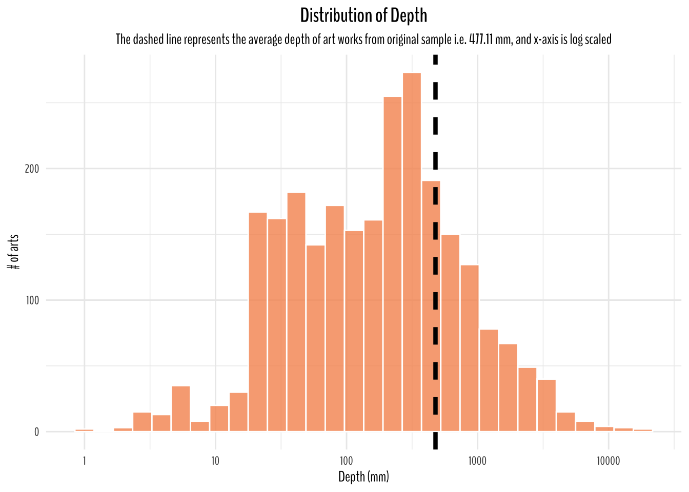
Since, I have assumed this dataset to be representative of all art works around the world. I think a good starting point to think of average dimension would be to calculate the averages from this dataset which is 346.88 mm in height, 323.81 mm in width, and 477.11 mm in depth.
Resampling
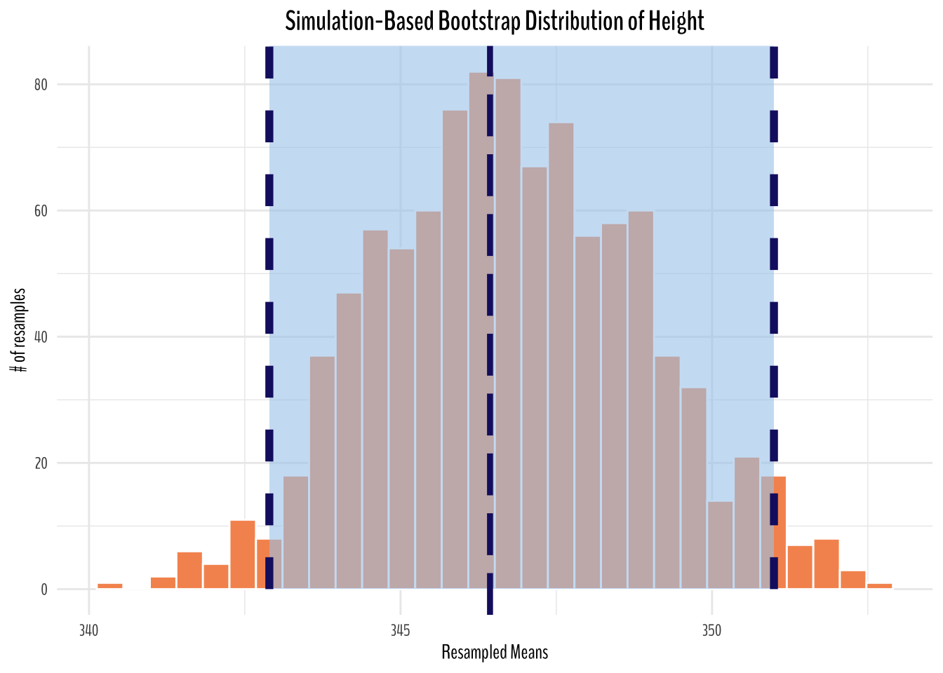
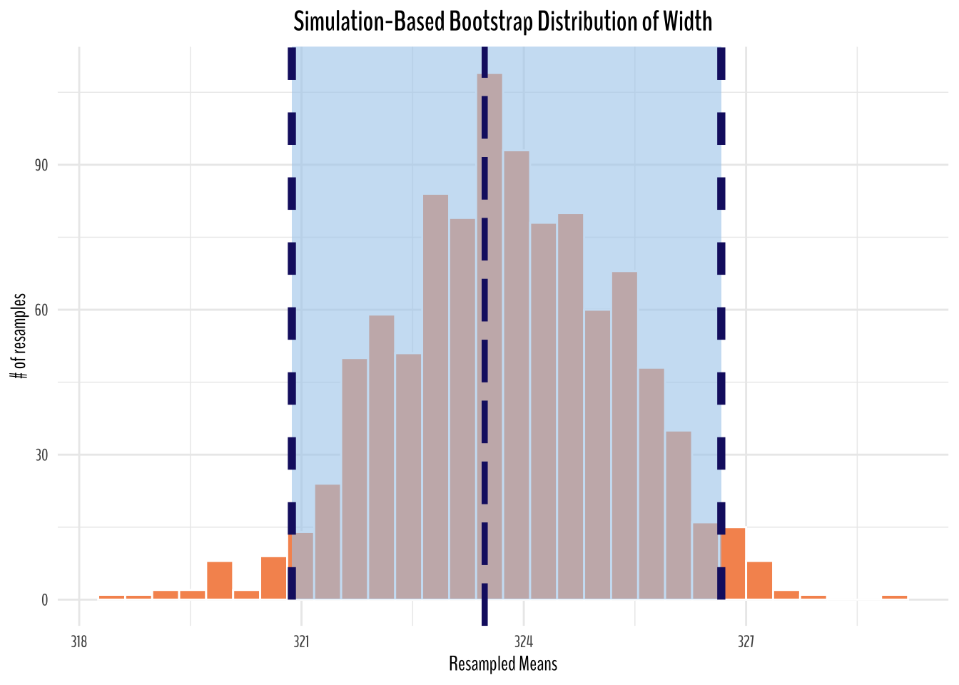
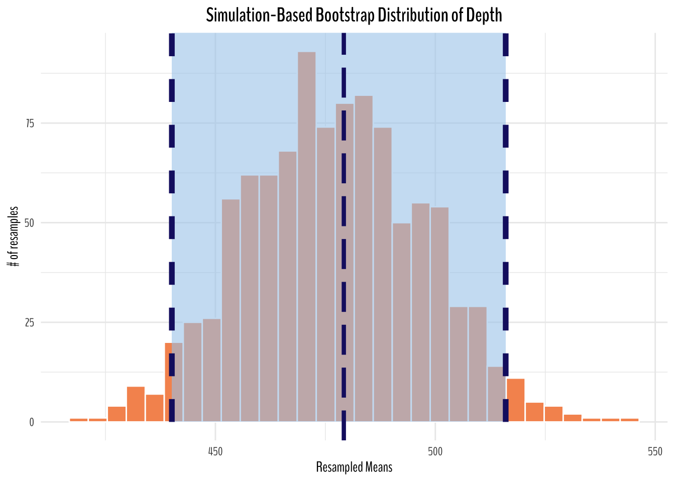
I will perform a 1000 bootstrap resample on my original sample which is this dataset and calculate averages on the resamples for height, width, and depth.
I am not going to get into explaining what confidence interval and p-values are. I think a good place to learn about them using this similar workflow would be Statistical Inference via Data Science. I would highly recommend checking out this book if you want to have a clear concept on standard error, confidence intervals, resampling, bootstraps, hypothesis testing, etc.
Bootstrap Distribution of Height
artwork_height_bootstrapped_means <- artwork_artist_tbl %>%
  filter(!is.na(height)) %>%
  rowid_to_column(var = "ID") %>%
  select(ID, height) %>%
  specify(response = height) %>%
  generate(reps = 1000, type = "bootstrap") %>%
  calculate(stat = "mean")
height_ci_endpoints <- artwork_height_bootstrapped_means %>%
get_ci()
artwork_height_bootstrapped_means %>%
ggplot(aes(stat)) +
geom_histogram(fill = "#F6955E", color = "white") +
shade_ci(
endpoints = height_ci_endpoints,
color = "midnightblue",
fill = "#A8CDEC",
linetype = "dashed"
) +
labs(title = "Simulation-Based Bootstrap Distribution of Height",
y = "# of resamples",
x = "Resampled Means") +
geom_vline(
xintercept = artwork %>% summarize(avg_height = mean(height, na.rm = T)) %>% pull(avg_height),
color = "midnightblue",
size = 1.5,
lty = 5
) +
theme_minimal() +
theme(
text = element_text(family = "BenchNine"),
plot.title = element_text(size = 15, face = "bold", hjust = 0.5)
)
Bootstrap Distribution of Width
artwork_width_bootstrapped_means <- artwork_artist_tbl %>%
  filter(!is.na(width)) %>%
  rowid_to_column(var = "ID") %>%
  select(ID, width) %>%
  specify(response = width) %>%
  generate(reps = 1000, type = "bootstrap") %>% # generating 1000 bootstrapped
  calculate(stat = "mean")
width_ci_endpoints <- artwork_width_bootstrapped_means %>%
get_ci()
artwork_width_bootstrapped_means %>%
ggplot(aes(stat)) +
geom_histogram(fill = "#F6955E", color = "white") +
shade_ci(
endpoints = width_ci_endpoints,
color = "midnightblue",
fill = "#A8CDEC",
linetype = "dashed"
) +
labs(title = "Simulation-Based Bootstrap Distribution of Width",
y = "# of resamples",
x = "Resampled Means") +
geom_vline(
xintercept = artwork %>% summarize(avg_width = mean(width, na.rm = T)) %>% pull(avg_width),
color = "midnightblue",
size = 1.5,
lty = 5
) +
theme_minimal() +
theme(
text = element_text(family = "BenchNine"),
plot.title = element_text(size = 15, face = "bold", hjust = 0.5)
)
Bootstrap Distribution of Depth
artwork_depth_bootstrapped_means <- artwork_artist_tbl %>%
  filter(!is.na(depth)) %>%
  rowid_to_column(var = "ID") %>%
  select(ID, depth) %>%
  specify(response = depth) %>%
  generate(reps = 1000, type = "bootstrap") %>% # generating 1000 bootstrapped
  calculate(stat = "mean")
depth_ci_endpoints <- artwork_depth_bootstrapped_means %>%
get_ci()
artwork_depth_bootstrapped_means %>%
ggplot(aes(stat)) +
geom_histogram(fill = "#F6955E", color = "white") +
shade_ci(
endpoints = depth_ci_endpoints,
color = "midnightblue",
fill = "#A8CDEC",
linetype = "dashed"
) +
labs(title = "Simulation-Based Bootstrap Distribution of Depth",
y = "# of resamples",
x = "Resampled Means") +
geom_vline(
xintercept = artwork %>% summarize(avg_depth = mean(depth, na.rm = T)) %>% pull(avg_depth),
color = "midnightblue",
size = 1.5,
lty = 5
) +
theme_minimal() +
theme(
text = element_text(family = "BenchNine"),
plot.title = element_text(size = 15, face = "bold", hjust = 0.5)
)
Conclusion
From the simulated plots above, we can see that if we were to repeat the same sampling procedure a large number of times, we expect about 95% of the intervals to capture the value of the true population parameter. In this case, we can see our original sample mean is captured in the 95% confidence interval (percentile method).